Machine Learning (ML) and Artificial Intelligence (AI) are well underway to becoming a staple in quantitative economics. Regularly, new fascinating applications hit national or international media. From AI outperforming doctors diagnosing breast cancer, over identifying dialects in naked mole rats to monitoring hiring discrimination, it seems no field is immune to the breakthroughs promised by AI. Similarly, a wide and expanding set of machine learning methods has been put forward. This poses challenges to researchers outside computer science wanting to incorporate such methods into their research.

Machine learning methods face an inherent trade-off between accuracy on the one hand, and computational burden and intelligibility on the other. To improve accuracy, methodological innovations are suggested that reduce interpretability for the researcher and require parameter optimization, often through running and comparing more models. In other words, increased predictive ability comes at a cost. In this blog post, I want to a highlight a relatively simple machine learning method that offers good out-of-the-box predictions: Cubist. Cubist was developed in the 1990s by J.R. Quinlan and has gained attention recently, partly due to the release of the R package Cubist (see here for a list of publications). Similar to Cubist artwork, where objects are broken up and reassembled, the Cubist algorithm breaks up prediction by first growing a decision tree and then building linear regression models associated with the terminal leaves. This approach combines the flexibility of a decision tree with the linear predictability of linear regression models.

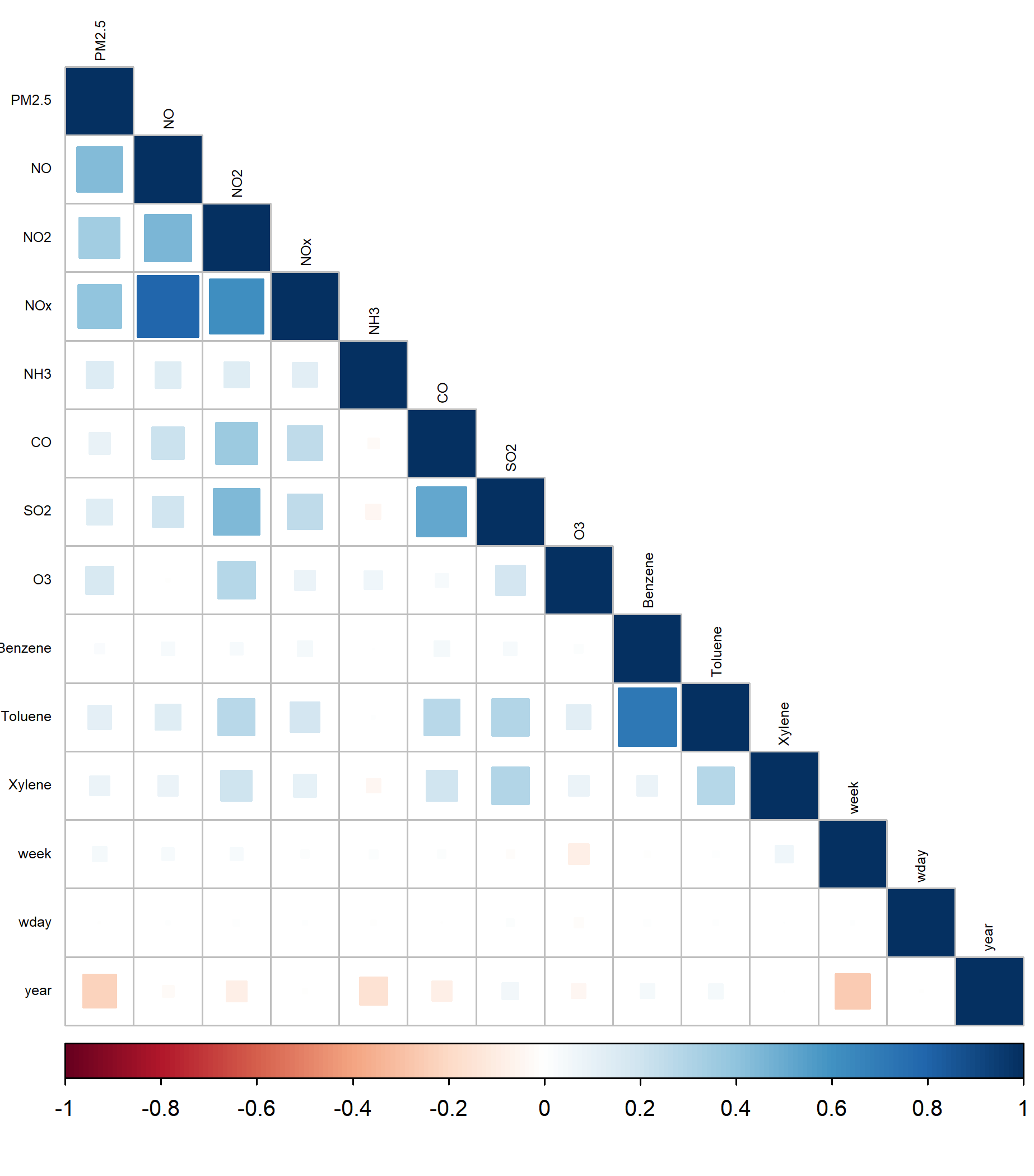
To highlight Cubist’s predictive ability, I will run a small comparative analysis inspired by Xu et al. (2018). Out dataset contains the concentration of fine particles that are two and one half microns or less in width (PM2.5) as the response variable and the concentration of several other chemicals, the city and date of measurement as explanatory variables (the date is transformed into year, day of the week and week of the year). Data are embedded here. The correlation plot below demonstrates moderate levels of correlation between the response variable and some predictor variables. Some related chemicals such as toluene and benzene show higher correlation levels.

To highlight Cubist’s relative strengths, I compare five different machine learning methods: (1) multiple linear regression (MLR), (2) Least Absolute Shrinkage and Selection Operator (LASSO), (3) Random forest (RF), (4) eXtreme Gradient Boosting (XGBoost), and (5) Cubist. I use cross-validation for LASSO for ease of prediction. The latter three approaches require optimising the number of iterations. For random forests, the only limitation is computational time as running more decision trees does not increase the chance of overfitting. Here, I use 1000 decision trees. For the Gradient Boosting and Cubist approaches, which are vulnerable to overfitting when too many iterations are run on the training data, the optimal number of iterations can be chosen by comparing the loss function for different values of the iterations using the test data. Using the root mean squared error (RMSE), I set 300 and 60 iterations for the Gradient Boosting and Cubist approaches, respectively. I also include the naive run with only one iteration. Lastly, I calculate a bagged model using weights to combine all optimised and the LASSO and MLR approaches. As optimisation criterium, the R squared was used.

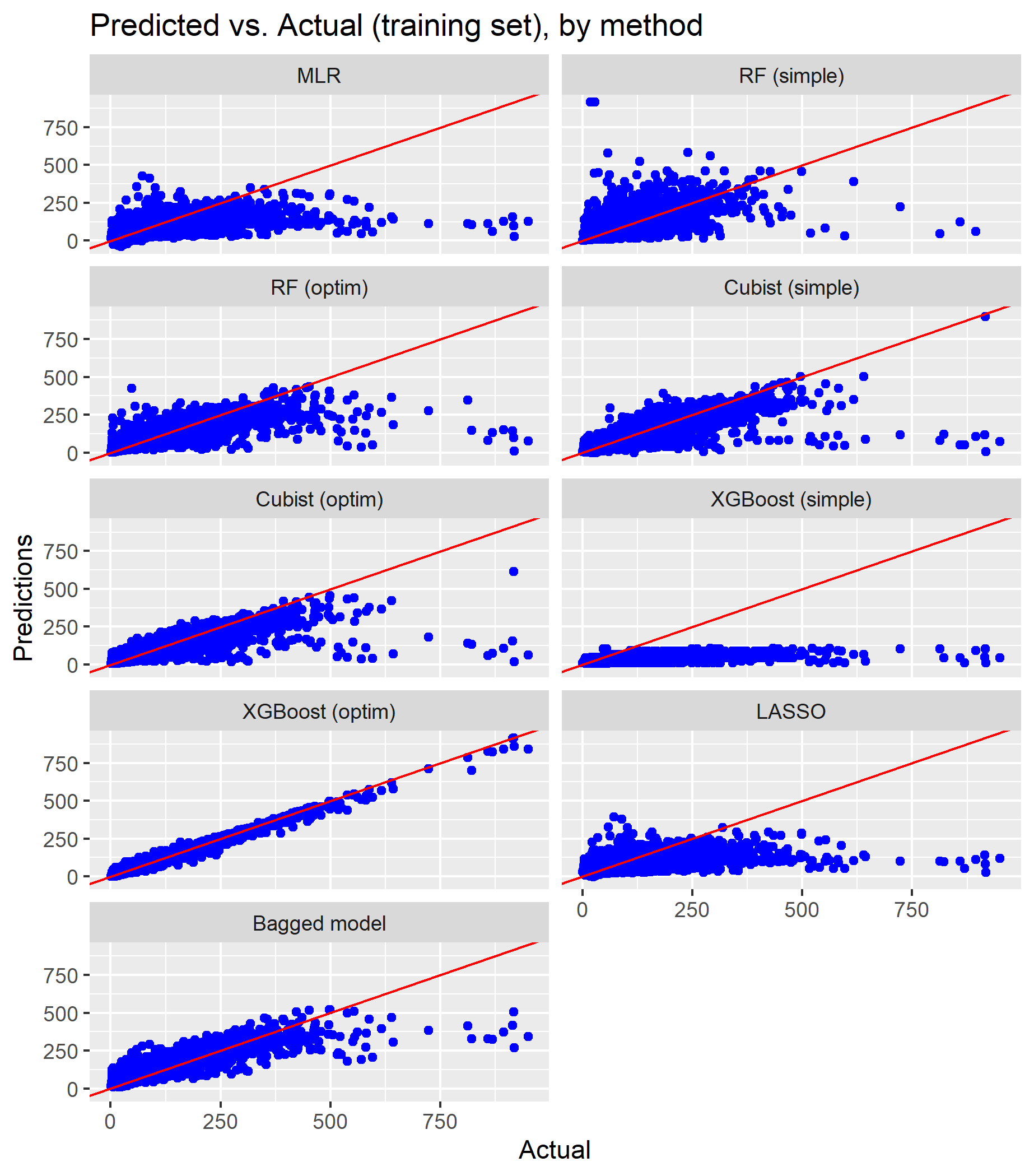
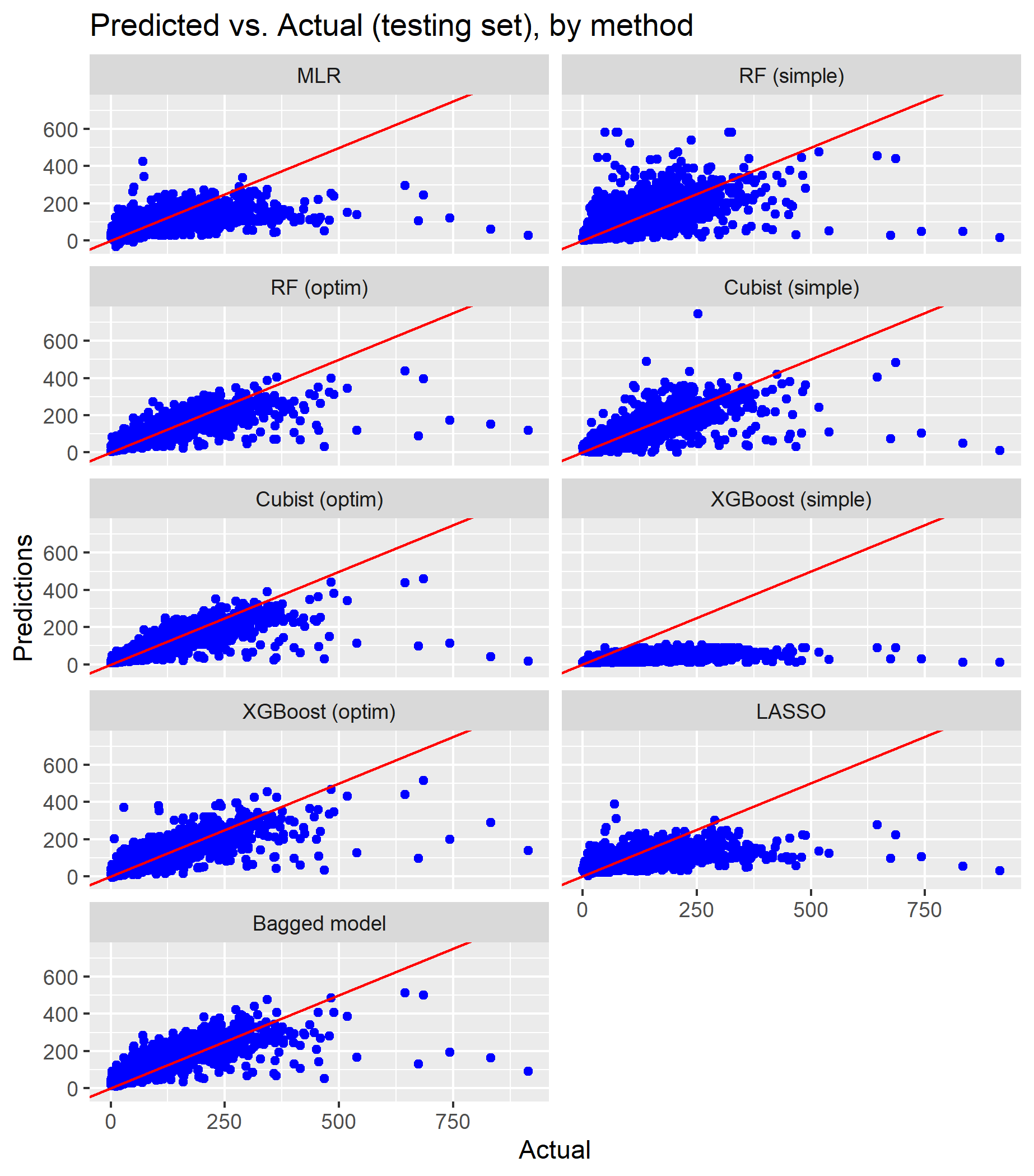
The figures below compare the fitted and true values for both the training set (used to train the models) and the test set (used to test the models).

To assess each method’s accuracy more formally, the table below lists three loss functions: the root mean squared error (RMSE), the mean absolute error (MAE) and the R squared (for both the training and Cross Validating (CV) using the test dataset).

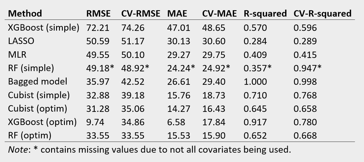
Although the exact ranking differs slightly, our results confirm those by Xu et al. (2018) (Table 2) by showing that the random forest, extreme gradient boosting and cubist approaches perform best with very similar performance levels. Interestingly, the naive Cubist performs only slightly worse than the optimised version, contrary to the naive extreme gradient boosting approach, which performs even worse than the linear regression. The bagged model performs very well in terms of R squared (for which it was optimised) but averagely for the other loss parameters. Although the naive Cubist model does not perform best, the lack of optimisation makes it significantly faster to compute. Given the trade-off between accuracy and computational burden mentioned in the beginning, naive Cubist’s minor loss in prediction accuracy when considering only one single iteration, seems a good deal. For researchers working with continuous outcome data, Cubist might act as a good initial exploratory model (see this blog post for a similar discussion). It’s quick, offers more interpretability than for example a random forest, and has good predictive performance.