In this blog I will discuss different approaches to adjust standard errors for panel data. As panel data often contains both a time and spatial dimension, considerations of serial and spatial correlation often require more than the standard heteroskedasticity-robust standard errors. A popular choice is clustering on the time, group or both levels; clustering on a supra-group level is also possible in case correlation between the groups might be problematic (see future blogs). Here I will restrict myself to clustering on the group level(s) and compare those results to the (less common) Newey–West and Driscoll–Kraay adjusted standard errors. Code (Stata) and data (Egger and Nelson, 2011) to reproduce the results can be found here.

1 Method

1.1 Empirical model

To set up our model we follow Egger and Nelson (2011) who employ an empirical gravity model for panel data. They include two sets of variables: antidumping measures and other trade frictions. The former consists of a count variable reflecting the number of antidumping investigations importing country j has initiated against exporting country i in year t (AD). Secondly, we use the cumulative number of antidumping investigations an economy j has launched against country i until year t (CAD). This would capture a possibly long memory in trade.

A second set of variables captures bilateral trade frictions. Since trade cost itself is not readily available, geographic distance and four measures of economic distance are used instead. Geographic distance is measured as bilateral great circle distances between two countries’ capitals (DIST). Economic distance includes a dummy variable that takes the value 1 in the absence of a common border and 0 otherwise (NBORD), a cultural (language) distance variable that is l in the absence of a common official language and 0 otherwise (NLANG), and two variables indicating (the absence of) common regional trade agreement membership for each country pair and year—one for customs unions (NCU) and the other one for free trade areas (NFTA).

Bilateral trade frictions are captured by exporter (CTY) and importer (PTN) fixed-effects dummies (Redding and Venables, 2004) as the time-invariant variables (distance, border and language) are of interest.

To complete the model, we add year-fixed-effects (YEAR) to control for macroeconomic shocks and a time trend (t) to proxy for technical progress. To reduce the problem of heteroskedasticity, we take the natural logarithm of both distance and the dependent variable (export volumes, X). Following Anderson and Van Wincoop (2004), we transform export volumes by subtracting importer and exporter GDP:

.

Our prime model of interest is the bilateral gravity model:

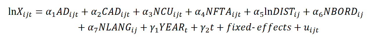
1.2 Estimation strategy

Heteroskedasticity and autocorrelation can be problematic in a panel setting. In fact, when the number of individuals (cross-sectional units, N) is large, using robust inference is considered good practice, even without testing for heteroskedasticity and autocorrelation. To adjust standard errors in a panel setting, different mechanisms exist. Under the assumption of independently (but not identically) distributed residuals, Eicker (1967), Huber (1967) and White (1980) propose standard errors that are robust to heteroskedasticity. An important drawback of these so-called White standard errors is the requirement that the number of time periods (T) is large (because the within transformation induces serial or temporal correlation) and no serial correlation is present (Stock and Watson, 2008).

To relax these assumptions, so-called Rogers or clustered standard errors are available (Arellano, 1987; Froot, 1989; Rogers, 1993). Clustered standard errors have gained considerable popularity in recent years because they not only allow for heteroskedasticity and serial correlation, but within-cluster correlation as well. However, requirements for correct implementation somewhat limit the potential of adjusting for spatial correlation through clustering.

Firstly, to allow for within-cluster correlation, no between-cluster correlation may be present and the number of clusters needs to be large (typically at least 20-50). The panel variable must also be nested within the cluster variable (again, because the within transformation induces serial correlation) (StataCorp, 2017). For the typical case of US firms or cities, clustering on the state- or industry-level is preferable due to likely correlation between firms or cities. Still, the number of industries or states might be too low (e.g. with unbalanced panels). Therefore, there is a latent trade-off in correct cluster-robust inference because larger cluster aggregation levels show less correlation but are also smaller in number.

Lastly, to allow for serial correlation, clustering on the panel ID level is needed (StataCorp, 2017). This, however, forces us the make the assumption that the disturbances are independently distributed over the panels (cluster level). Thus, a second trade-off emerges: when using clustering to adjust for serial correlation, no cross-sectional correlation is allowed. Lastly, to account for serial correlation, the number of individuals must be substantially larger than the number of time periods (Wooldridge, 2013).

Focusing on the issue of heteroskedasticity and autocorrelation, consistent standard errors can also be obtained by the Newey-West procedure (Newey and West, 1987). Contrary to previous approaches that allow for general patterns of serial correlation (including no pattern), the Newey-West method requires specification of the number of time lags. Essentially, this estimator is an extension to White standard errors and Newey–West standard errors with lag length zero will collapse to White standard errors.

Previous approaches have ignored the possibility of errors being correlated across (groups of) individuals (cross-sectional or spatial dependence). A practical way around this is to assume that the cross-sectional correlations are identical for every pair of individuals. Under this assumption, time-fixed-effects (dummies) capture and thus remove the spatial dependence (Hoechle, 2007). Alternatively, Driscoll and Kraay (1998) proposed a more general procedure. The corresponding Driscoll-Kraay or spatial correlation consistent (SCC) standard errors are robust to general forms of both spatial and serial dependence. A drawback of Driscoll-Kraay standard errors is their reliance on large-T asymptotic theory.

Lastly, we can also use bootstrapping as a general way of correcting standard errors. However, as bootstrapping assumes (spatial and serial) independence, the simple random bootstrap is not expected to improve the standard errors much (Dixon, 2001). Instead, bootstrapping is performed on clustered standard errors. With this type of bootstrapping, every sample drawn during each replication is a bootstrap sample of clusters and a new variable containing an unique identifier for each resampled cluster is required.

1.3 Data

The data used in this analysis was taken from the online repository for the Review of Economics and Statistics (Harvard Dataverse). More specifically, we used the dataset as compiled by Egger and Nelson (2011) for their study on the effects of antidumping on trade. We refer to their publication for more information on the variables used.

2 Results & discussion

Note that the distance effect in the country fixed-effects model is positive and non-significant while it is usually negative and significant (Disdier and Head, 2008). This result might be due to a lack of geographic representation in the dataset—for example, Germany has as many export partners (over the years) as Grenada, which seems implausible.

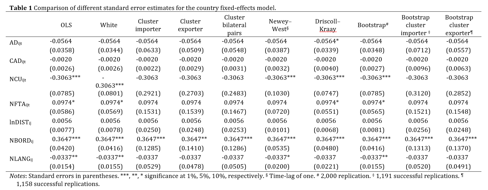
Table 1 presents standard errors for the country fixed-effects model using different adjustment mechanisms. In general, the non-clustered standard errors differ only slightly from the unadjusted (OLS) errors. The clustered errors—whether using importer, exporter or bilateral pairs as cluster level, and whether bootstrapped or not—however, are several times higher than de OLS errors. Consequently, the variables NLANG, NCU and NFTA lose their significance using the clustered standard errors. Assuming the OLS errors are biased due to heteroskedasticity and serial correlation, the small differences with the White, Newey–West, Driscoll–Kraay and simple bootstrap adjusted errors, are problematic. The White and simple bootstrap standard errors were not expected ex ante to perform well. The failure of the Newey–West errors might be due to the higher-lag nature of the serial correlation while that of the Driscoll–Kraay errors may be caused by its reliance on large T samples. Due to the low number of supranational regions (e.g. continents), we did not cluster on an aggregated level—if spatial autocorrelation is a serious concerns, spatial panel models are preferred. Driscoll–Kraay standard errors could in theory help to solve spatial autocorrelation. In this application, however, the Driscoll–Kraay adjustment does not seem to work well, again possibly due to its reliance on large T samples.

3 References

Anderson, J.E., Van Wincoop, E., 2004. Trade costs. Journal of Economic literature 42, 691–751.
Arellano, M., 1987. Computing Robust Standard Errors for Within‐groups Estimators. Oxford bulletin of Economics and Statistics 49, 431–434.
Disdier, A.-C., Head, K., 2008. The puzzling persistence of the distance effect on bilateral trade. The Review of Economics and statistics 90, 37–48.
Dixon, P.M., 2001. The bootstrap and the jackknife. Design and analysis of ecological experiments 267–288.
Driscoll, J.C., Kraay, A.C., 1998. Consistent covariance matrix estimation with spatially dependent panel data. Review of economics and statistics 80, 549–560.
Egger, P., Nelson, D., 2011. How bad is antidumping? Evidence from panel data. Review of Economics and Statistics 93, 1374–1390.
Eicker, F., 1967. Limit theorems for regressions with unequal and dependent errors, in: Proceedings of the Fifth Berkeley Symposium on Mathematical Statistics and Probability. pp. 59–82.
Froot, K.A., 1989. Consistent covariance matrix estimation with cross-sectional dependence and heteroskedasticity in financial data. Journal of Financial and Quantitative Analysis 24, 333–355.
Hoechle, D., 2007. Robust standard errors for panel regressions with cross-sectional dependence. Stata Journal 7, 281.
Huber, P.J., 1967. The behavior of maximum likelihood estimates under nonstandard conditions, in: Proceedings of the Fifth Berkeley Symposium on Mathematical Statistics and Probability. Berkeley, CA, pp. 221–233.
Newey, W.K., West, K.D., 1987. A simple, positive semi-definite, heteroskedasticity and autocorrelation consistent covariance matrix. Econometrica 55, 703–708.
Redding, S., Venables, A.J., 2004. Economic geography and international inequality. Journal of international Economics 62, 53–82.
Rogers, W.H., 1993. sg17: Regression standard errors in clustered samples. Stata technical bulletin 13, 19–23.
StataCorp, 2017. Stata 15 Base Reference Manual. Stata Press, College Station, TX.
Stock, J.H., Watson, M.W., 2008. Heteroskedasticity‐robust standard errors for fixed effects panel data regression. Econometrica 76, 155–174.
White, H., 1980. A heteroskedasticity-consistent covariance matrix estimator and a direct test for heteroskedasticity. Econometrica: Journal of the Econometric Society 817–838.
Wooldridge, J.M., 2013. Introductory econometrics: a modern approach, 5th ed. South-Western Publishing, Mason, OH.